How to Build a Graph Convolutional Network with JAX and Equinox!

02 Sep 2024

I’ve been learning JAX for the past few months and for a recent project I needed to train a basic Graph Neural Network. Surprisingly, I couldn’t find good libraries to easily build GNNs. Most of them are outdated and don’t use my DL framework of choice (Equinox!). This was the perfect excuse to implement my own GNNs from scratch.

I love the JAX/Equinox combination. In my opinion it is perfect for DL research. It gives the user an approachable low-level API that they can play with and that scales well thanks to its powerful JIT compiler. If you’re not already using JAX, have a look at long live JAX.

So let’s dive in. We’ll see the simplest implementation first using the adjacency matrix of the graph. Then, we’ll continue with the more complex but modular approach using the edge list representation.

Level 1: Using the Adjacency Matrix

Let’s first recap how we usually represent a graph. For a list of $N$ nodes, we represent the relation between the nodes with an adjacency matrix $A \in \mathbb{N}^{N \times N}$ where $a_{i, j} \in \{0, 1\}$ represents the edge from node $j$ to node $i$ ( $1$ if the edge actually exists, $0$ otherwise). We use this adjacency matrix to summarize how the nodes are connected to each other.

Each node being represented by some vector of size $H$ , we can represent the set of nodes as a matrix in $\mathbb{R}^{N \times H}$ . This lets us write our first graph convolutional layer:

import jax.experimental.sparse as jsparse


class GraphConv(eqx.Module):
    linear: nn.Linear

    def __init__(self, hidden_dim: int, *, key: PRNGKeyArray):
        self.linear = nn.Linear(hidden_dim, hidden_dim, key=key)

    def __call__(
        self,
        nodes: Float[Array, "n_nodes hidden_dim"],
        adjacency: Int[jsparse.BCOO, "n_nodes n_nodes"]
    ) -> Float[Array, "n_nodes hidden_dim"]:
        messages = vmap(self.linear)(nodes)
        return adjacency @ messages

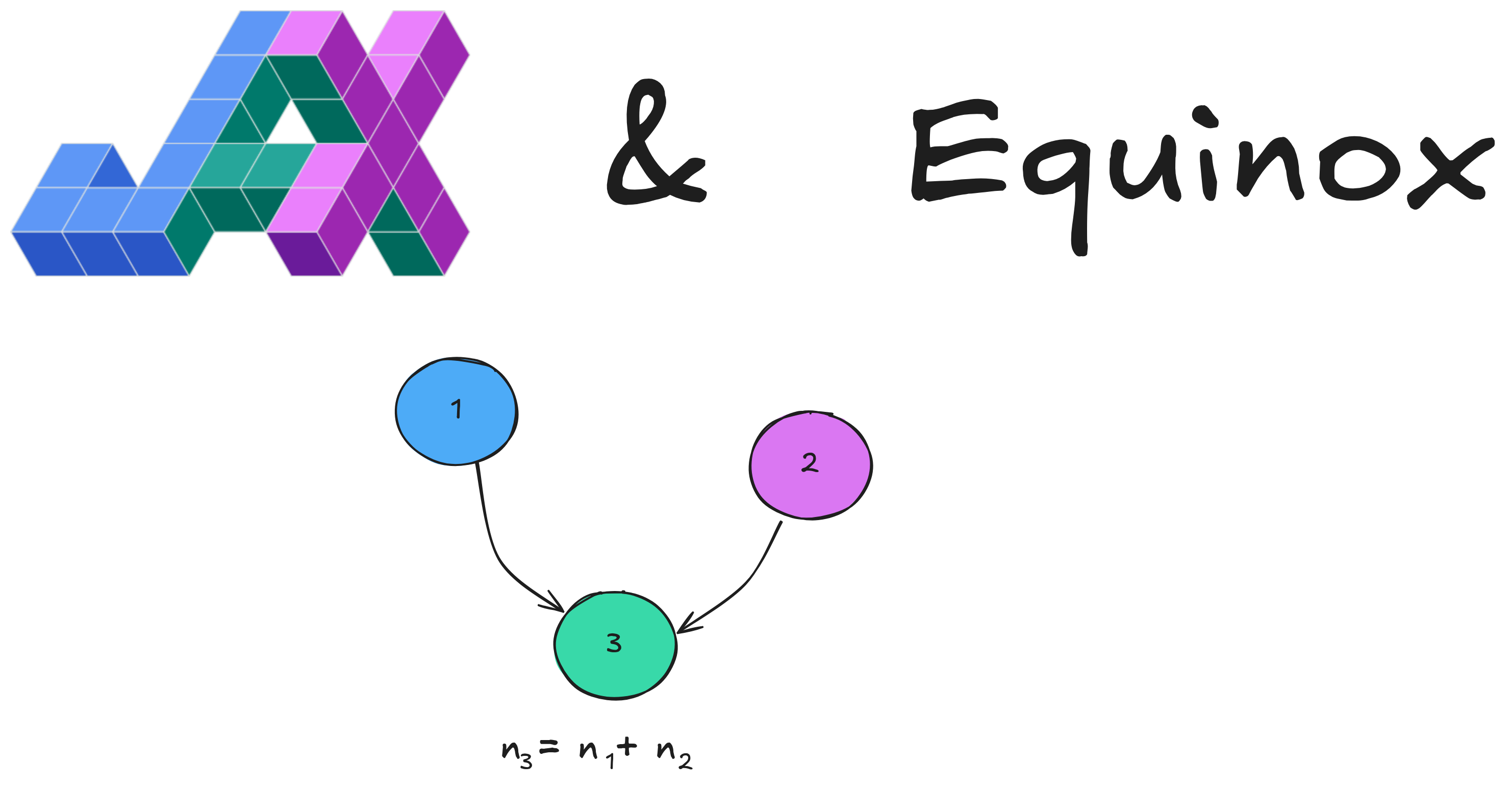
Doing this matrix multiplication between the node representation and the adjacency matrix is equivalent to the following computation:

n_i^{k+1} = \sum_{j \in \mathcal{N(i)}} W n_j^k

Where $n_i^k \in \mathbb{R}^H$ is the hidden representation of the node $i$ at layer $k$ and $\mathcal{N(i)}$ is the set of neighbours of the node $i$ .

Essentially, each node’s representation is updated by taking the sum of its neighbours’ after applying a linear transformation. You can see how using the adjacency matrix makes it easy.

To be computationally efficient, we use the sparse matrix multiplication of JAX. Note that at the time of writing this article, this module is still experimental.

Level 2: Using the Edge List

Even though the adjacency matrix is an efficient and concise way to implement the graph convolutional layer, it can be hard (impossible?) to define other classical graph layers. That’s why we often use another representation of our graph: the edge list.

We use a tensor $E \in \mathbb{N}^{M \times 2}$ where $e_k = (j, i)$ indicates that the $k^{th}$ edge is an edge from node $j$ to node $i$ (for a total of $M$ edges). With this, we can reproduce the previous implementation:

class GraphConv(eqx.Module):
    linear: nn.Linear

    def __init__(self, hidden_dim: int, *, key: PRNGKeyArray):
        self.linear = nn.Linear(hidden_dim, hidden_dim, key=key)

    def __call__(
        self,
        nodes: Float[Array, "n_nodes hidden_dim"],
        edges: Int[Array, "n_edges 2"],
    ) -> Float[Array, "n_nodes hidden_dim"]:
        messages = vmap(self.linear)(nodes)
        messages = messages[edges[:, 0]]  # Shape of [n_edges hidden_dim].
        messages = jax.ops.segment_sum(
            data=messages,
            segment_ids=edges[:, 1],
            num_segments=len(nodes),
        )  # Shape of [n_nodes hidden_dim].
        return messages

This is much less intuitive! Let’s break this down.

First, we apply the linear layer to all nodes just as we did previously. Then, the embeddings are copied and reordered to align with the sources of the edges. At this point, we have the list of all features coming from each source node $j$ of $e_k = (j, i)$ . Finally, those features are aggregated with respect to the destination nodes $i$ .

This last step uses jax.ops.segment_sum, which does exactly what we want and frees us from complex gather and scatter operations. It takes a list of multiple vectors and selectively adds them based on the corresponding segmend_ids list (the destination ids in our case).

Once we understand what this function does it becomes easy to read and tweak the code to our needs. As an additional example, here is how we could compute the degree of all nodes:

ones = jnp.ones(len(edges), dtype=jnp.int32)
degrees = jax.ops.segment_sum(
    data=ones,
    segment_ids=edges[:, 1],
    num_segments=len(nodes),
)

This should be easily understandable.

The significant advantage of this representation is that it allows for more flexibility.

By looking at the jax.ops documentation, we can see that we have access to other operations such as segment_min and segment_max. Different segment operations will change the aggregation scheme.

Additionally, we can now apply a linear transformation on the edges. By concatenating the source and destination features, we can apply the linear layer such that it takes into account both pieces of information. If edge features are available, it could be used here as well.

Note that if an id is not present in the segment_ids list, it will be filled with a default value that is specific to the segment operation used. For instance, segment_sum will fill any missing destination id with 0s whereas segment_min will fill them with inf values.

Training the Models

So to test everything, I’ve set up a fictive ranking task. Random graphs are generated using networkx and some score is given to each node according to the clustering metric.

Two different GNNs are trained using a ranking loss applied to the nodes. The first model is the classical GCN using the adjacency representation. The second is an implementation of GAT, a more complex GNN, implemented using the edge list representation.

You can find the code here. The two models are trained on 800 random graphs with 100 nodes and about 600 edges each. They have ~170,000 parameters and are trained for 50 000 steps. On my GTX 1080 it took about 40 minutes for the GCN and 50 minutes for the GAT.

So here’s how the training went:

Validation scores on andom graphs

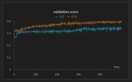
I use the Kendall ranking metric, which measures how much the ranking provided by the models is correlated with the actual ranking of the nodes. A perfectly predicted rank would have a score of $1$ .

Sadly, for this fictive task, it looks like the basic GCN is more effective than GAT. Anyway, the goal was to have a concise implementation somewhere that I (and you maybe) can reuse for future works.

JIT Tips

When using JAX, it is crucial to JIT your computations. The way JIT works is that the first time it encounters your function, it will compile it and keep a cache of the compilation so that later on when you call the same function again it can just use the cached compilation directly.

But the cached version of your function is shape-dependent, meaning that if you pass an argument with a different shape, it will need to recompile everything and cache the new result again. This is an issue for our graphs because we typically have a variable number of nodes and edges for different graphs of our datasets.

It means that in order to avoid recompilation, we need to pad our graphs before feeding them into the model. For the adjacency matrix, we can simply fill it with more 0s. For the edge list, we can create fictive self-loops to a padded fictive node.

You can have a look at this explanation from a JAX dev for a more in-depth understanding of how JIT works under-the-hood.

Final Thoughts

While the adjacency representation makes it easy to define the classical GCN, it is less customizable. The second implementation, using the edge list, is flexible and allows for more complex GNNs. Nervertheless, keep in mind that the adjacency representation remains more computationally efficient and requires less memory.

You can have a look at the whole code used to train the models here: gnn-tuto.